A second level of introduction of physical properties was proposed by Godunov (1959) [6]. This method and all its generalisations and extensions are sometimes referred as flux-difference splitting methods or Godunov-type methods. At the expenses of increasing the complexity of the scheme and the computational effort required to perform calculation, the exact approximate local properties of basic solutions to the Euler equations can be directly introduced in the discretization strategy. Rather than attempting to follow characteristics backward in time (like in the CIR method), Godunov suggested solving Riemann problems forward in time. The Godunov's scheme can be defined in three main steps:
 ;
;
 are obtained
by averaging the local solution inside each cell;
are obtained
by averaging the local solution inside each cell;
The update in Godunov-type schemes is done on the cell-averaged
conservative variables. The update requires estimation of numerical
fluxes at cell-interfaces and a successive integration in time over a
time-step. Hence, the first step of the Godunov scheme
approximates the point-values of
the solution at each interface by a piecewise-constant reconstruction.
The values of the conservative variables at a grid point
are considered as a piecewise-constant approximation of the true
solution over the cell centered at that grid point.
The piecewise-constant approximation defined at this step is a cell-average
of the solution, so the spatial error is of the same order of the cell
size  and the scheme is only first-order accurate in space.
Several high-order accurate generalizations of this scheme have been
proposed based on high-order polynomial reconstructions of
pointwise values from cell-averaged values.
Let us indicate in the following this step by the application
of the operator
and the scheme is only first-order accurate in space.
Several high-order accurate generalizations of this scheme have been
proposed based on high-order polynomial reconstructions of
pointwise values from cell-averaged values.
Let us indicate in the following this step by the application
of the operator  to the ensemble of the cell-averaged state-values
 representing the solution at time
  . Hence,
 will represent the high-order accurate
polynomial approximation inside any cell of the computational domain at time
will represent the high-order accurate
polynomial approximation inside any cell of the computational domain at time
 .
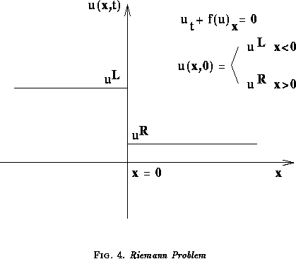
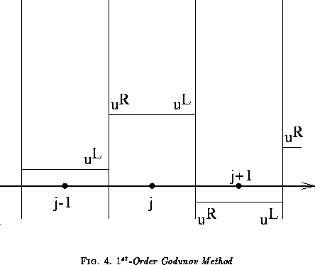
This reconstruction produces a discontinuity in the state variables at
each interface which is taken as initial condition for a particular
initial value problem called Riemann problem, where a one-dimensional
conservation law or system of conservation laws like
.
This reconstruction produces a discontinuity in the state variables at
each interface which is taken as initial condition for a particular
initial value problem called Riemann problem, where a one-dimensional
conservation law or system of conservation laws like

is considered with an initial solution of the type:
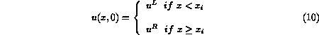
The initial data at time  is piecewise-constant and is characterized
by the two states
is piecewise-constant and is characterized
by the two states  and
and  respectively on the left (
 )
and on the right
)
and on the right  of the position
  , where the discontinuity
is located.
, where the discontinuity
is located.
In the case of Euler equations this problem has always a
solution and the algorithm which solves it is called a Riemann solver,
see LeVeque (1990) [14]. Let us formally denote this step by the
application of the operator  (evolution through a time
interval
(evolution through a time
interval  ). The solution of the Riemann problem allows us
to introduce in a very direct and natural way a knowledge of the
propagation and interactions of nonlinear waves, locally described by
the Riemann solver. The constant state used as input to the Riemann
solver are chosen to represent the domains of dependence for the
cell-interface which is swept out during the time-step
). The solution of the Riemann problem allows us
to introduce in a very direct and natural way a knowledge of the
propagation and interactions of nonlinear waves, locally described by
the Riemann solver. The constant state used as input to the Riemann
solver are chosen to represent the domains of dependence for the
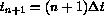
cell-interface which is swept out during the time-step
 by the different families of characteristic
curves of the Euler equations. The information contained in these
domains of dependence is given by the piecewise-polynomial
approximation describing the flow distribution inside any cell.
The solution can be built as a superposition of the elementary
waves locally satisfying the conservation equations, and this
estimate gives the cell-interface fluxes, or the numerical fluxes
can be directly given by some appropriate linearisation of the
Riemann problem. The Riemann solver computes the non-linear
interaction of two constant states of the fluid, and which
non-linear waves emerge from this interaction providing the
numerical discretization with a naturally upwind and non-linear
character. Finally, the solution at time
by the different families of characteristic
curves of the Euler equations. The information contained in these
domains of dependence is given by the piecewise-polynomial
approximation describing the flow distribution inside any cell.
The solution can be built as a superposition of the elementary
waves locally satisfying the conservation equations, and this
estimate gives the cell-interface fluxes, or the numerical fluxes
can be directly given by some appropriate linearisation of the
Riemann problem. The Riemann solver computes the non-linear
interaction of two constant states of the fluid, and which
non-linear waves emerge from this interaction providing the
numerical discretization with a naturally upwind and non-linear
character. Finally, the solution at time  is averaged in
space to yields the averaged-state variable
is averaged in
space to yields the averaged-state variable  . We will
represent this average by the application of a cell-average operator
. We will
represent this average by the application of a cell-average operator
 where
where  is the cell size.